2 Training and evaluating regression models
2.1 Model training
The goal of machine learning models such as regression is to predict the dependent variable, \(y\). For example, in the house pricing data set described in chapter 1, we defined as the dependent variable “SalePrice”, and as independent variables MSSubClass, MSZoning and the others in the data set.
\[SalePrice=\beta_{0}+\beta_{1}\ MSSubClass + \beta_{2}\ MSZoning+ ....+x_{n}+ e\]
where \(e\) is the error term. The regression model aims to estimate the parameters \(\beta_{1}, \beta_{2},...,\beta_{n}\), to predict SalePrice. The following would be the predicted model. We call that the training.
\[\hat{SalePrice}=\hat{\beta_{0}}+\hat{\beta_{1}}MSSubClass+\hat{\beta_{2}}MSZoning+....+\hat{\beta_{n}}x_{n} \]
The hat on the parameters indicates that these are estimated parameters. Note: When we are learning ML, it is convenient to understand what the models are doing step by step. If you are familiar with estimating the regression and prediction, you can skip the following steps until the Training and test set (Back testing).
To exemplify how ML in regression models works, we first estimate two independent variables: MSSubClass and MSZoning.
\[SalePrice=\beta_{0}+\beta_{1}\ MSSubClass + \beta_{2}\ MSZoning + \epsilon \]
house<-read.csv("data/house_clean.csv")
#house<-read.csv("https://raw.githubusercontent.com/abernal30/ml_book/main/housing.csv")
In R, we use the “lm” function to run the regression model by Ordinary Least squares
house_model<-lm(SalePrice~MSSubClass+MSZoning,data=house)
summary(house_model)
#>
#> Call:
#> lm(formula = SalePrice ~ MSSubClass + MSZoning, data = house)
#>
#> Residuals:
#>     Min      1Q  Median      3Q     Max
#> -169125  -58658  -26555   43751  532828
#>
#> Coefficients:
#>             Estimate Std. Error t value Pr(>|t|)
#> (Intercept) 354837.1    30654.8  11.575  < 2e-16 ***
#> MSSubClass    -233.4      102.0  -2.289   0.0224 *
#> MSZoning    -29665.2     7528.4  -3.940 9.12e-05 ***
#> ---
#> Signif. codes:  0 '***' 0.001 '**' 0.01 '*' 0.05 '.' 0.1 ' ' 1
#>
#> Residual standard error: 90790 on 581 degrees of freedom
#> Multiple R-squared:  0.03625,    Adjusted R-squared:  0.03294
#> F-statistic: 10.93 on 2 and 581 DF,  p-value: 2.194e-05
As a result, we get the following estimated model:
\[`\hat{r con[2]`}= 354837.1+-233.4\ MSSubClass + -29665.2\ MSZoning\]
In Machine Learning (ML), we are not concerned about the coefficient significance; in chapter one, we explain the differences between Machine Learning models and the causality approach ones where we explain that. In ML models, we predict the dependent variable, in this case, SalePrice, given certain features or independent variables.
Suppose we want to predict SalePrice for the values of the variables MSSubClass and MSZoning of 20 and 4, respectively. The following formula predicts SalePrice by taking the parameters of the OLS regression:
SalePrice=354837.1+354837.1 * 20+-29665.2*4 = 231508.1
The result 231508.1 predicts SalePrice when variables MSSubClass and MSZoning take the values of 20 and 4, respectively.
Remember that the previous result is for exposition proposes. We could use the “predict” function, which gives us the same result. We must add the arguments for the OLS model object and a data frame with the features we want to predict.
predict(house_model,house_test)
#>        1
#> 231508.1
We are still determining if the previous prediction is good. For the moment, we can compare with an observation in the “house” data set, for example, the first one:
head(house[1,2:4])
#>   SalePrice MSSubClass MSZoning
#> 1    181500         20        4
Our prediction is far from the SalePrice observation in the “house” data set. Of course, we need to add more independent variables and do some other procedures, which we will cover in subsequent sections.
2.1.1 Training and test set (Back testing)
In the previous section, we only made one prediction and compared it with a given observation. In the machine learning literature is common to apply that testing procedure for several observations. In this book, we call this back-testing, which divides the data set into training and testing, often called in_sample and out_sample. As in the previous example, the house_test must be a data frame. However, instead of having only one observation and two independent variables, it will contain many other observations and independent variables.
To answer why we need a back-testing, think that if we want to validate the prediction performance, we have at least two alternatives:
Alternative 1: Estimate a ML model, make a prediction and wait in time, for example, 30 days, to verify if the prediction is good or not; if the forecast is not good (it is not close to the real value), then we have to train and test it again, let’s say other 30 days and so on.
Alternative 2 (The one we will apply): Take aside some observations, assuming those are observations we don’t know and store them in a data frame called “test.” Train and test the ML model. If we are not making a good prediction, we train and test the model again until we get a good prediction performance.
It is a common practice to divide the data set into training (80% of the observations) and testing (the other 20%). However, other authors suggest splitting it into Training Set, Validation Set and a Test Set (Lantz 2019). In the latter case, the proposal is to train the model on the training set (for example, 60% of the data), do the cross-validation (a procedure we will cover below) on the validation set (for example, 20% of the data), and once the model has a good prediction performance, test it in the test set (20% of the data).
In this book, we will use both methods. We start in this chapter with the first one, and in the cross-validation chapter, we will cover the second one.
For the housing prices data set, we split randomly into 80%, applying the function sample.
set.seed (26)
dim<-dim(house)
train_sample<-sample(dim[1],dim[1]*.8)
house_train <- house[train_sample, ]
house_test  <- house[-train_sample, ]
The “set.seed” function helps us to control the results by getting the same aleatory partition in the data; otherwise, we would get a different result every time we run the R chunk. The spirit of this book is to compare various methods and methodologies without concern about the possible differences in the models or processes that result from the random partition.
head(house_train[,1:5])
#>      Id SalePrice MSSubClass MSZoning LotFrontage
#> 64   64    163000         20        4          80
#> 540 540    170000         80        4         102
#> 200 200    155000         70        5          50
#> 171 171    142000         20        4          65
#> 41   41    250000         60        2          75
#> 268 268    155000         60        4          70
If we compare the original house data set with the previous output, the “rownames” (or ID) are different and are not in order because they were selected randomly. Another important distinction is that the observations in the house_test data set complement the house_train. In other words, the observations (IDs) in the training set aren’t in the test, and vice versa.
head(house_test[,1:5])
#>    Id SalePrice MSSubClass MSZoning LotFrontage
#> 17 17    165500         20        4          70
#> 20 20    153000         20        4          74
#> 26 26    385000         20        4          68
#> 31 31    317000         60        4          76
#> 42 42    190000         20        4         105
#> 43 43 383970 60 4 772.1.3 RMSE
In the previous section, we discussed whether the prediction was good (the prediction performance). This section formally defines the metrics for the prediction performance.
The first metric is the Root Mean Square Error (RMSE). The mathematical formula to compute the RMSE is:
\[RMSE =\sqrt{\frac{1}{n}\ \sum_{i=1}^{n} (y_{i}-\hat{y_{i}})^{2}} \]
where \(\hat{y_{i}}\) is the prediction for the ith observation, \(y_{i}\) is the ith observation of the independent variable we store in the test set, and n is the number of observations.
\[\hat{y_{i}}=\hat{\beta_{0}}+\hat{\beta_{1}}x_{1}+,..,+\hat{\beta_{n}}x_{n}\]
We can estimate the RMSE using the training data set. But generally, we do not care how well the model works on the training set. Rather, we are interested in the model performance tested on unseen data; then, we try the RMSE on the test data set or the validation set for cross-validation. The lower the test RMSE, the better the prediction.
We estimate the RMSE for the housing example. This time we use all the variables in the data set. To train the model, we use the training data set. The “lm” function requires adding a dot after the symbol “~.”
house_model<-lm(SalePrice~.,data=house_train)
summary(house_model)
#>
#> Call:
#> lm(formula = SalePrice ~ ., data = house_train)
#>
#> Residuals:
#>     Min      1Q  Median      3Q     Max
#> -311484  -19921   -1159   18474  219630
#>
#> Coefficients:
#>                 Estimate Std. Error t value Pr(>|t|)
#> (Intercept)    1.535e+06  3.384e+06   0.454  0.65040
#> Id            -1.208e+01  1.268e+01  -0.953  0.34119
#> MSSubClass    -2.860e+02  1.367e+02  -2.092  0.03706 *
#> MSZoning      -1.286e+03  4.747e+03  -0.271  0.78667
#> LotFrontage   -3.126e+02  1.021e+02  -3.061  0.00235 **
#> LotArea        5.531e-01  2.113e-01   2.618  0.00918 **
#> LotShape      -2.770e+03  1.680e+03  -1.649  0.09984 .
#> LotConfig     -1.144e+03  1.422e+03  -0.805  0.42134
#> Neighborhood   3.287e+02  4.110e+02   0.800  0.42439
#> Condition1    -1.679e+03  2.579e+03  -0.651  0.51547
#> BldgType       1.202e+03  4.281e+03   0.281  0.77909
#> HouseStyle    -2.336e+03  1.830e+03  -1.276  0.20267
#> OverallQual    1.797e+04  3.096e+03   5.806 1.28e-08 ***
#> OverallCond    9.543e+03  2.960e+03   3.224  0.00136 **
#> YearRemodAdd  -1.525e+01  2.074e+02  -0.074  0.94142
#> RoofStyle      3.244e+03  2.784e+03   1.165  0.24465
#> Exterior1st   -1.142e+03  7.714e+02  -1.481  0.13937
#> MasVnrType     1.049e+03  3.500e+03   0.300  0.76450
#> MasVnrArea     5.071e+01  1.210e+01   4.189 3.42e-05 ***
#> ExterQual     -8.256e+03  4.918e+03  -1.679  0.09400 .
#> ExterCond      6.708e+02  3.758e+03   0.178  0.85842
#> Foundation     7.901e+03  5.232e+03   1.510  0.13179
#> BsmtQual      -1.073e+04  3.331e+03  -3.222  0.00137 **
#> BsmtExposure  -5.919e+03  2.114e+03  -2.801  0.00534 **
#> BsmtFinType1  -3.214e+03  1.588e+03  -2.024  0.04361 *
#> BsmtFinSF1    -2.507e+01  9.435e+00  -2.657  0.00819 **
#> BsmtUnfSF     -1.827e+01  9.992e+00  -1.828  0.06825 .
#> HeatingQC     -6.688e+02  1.636e+03  -0.409  0.68287
#> CentralAir     4.803e+03  2.020e+04   0.238  0.81217
#> Electrical     7.323e+02  3.113e+03   0.235  0.81414
#> X1stFlrSF      3.447e+01  1.291e+01   2.671  0.00786 **
#> X2ndFlrSF      2.999e+01  1.101e+01   2.724  0.00672 **
#> BsmtFullBath   1.070e+04  6.443e+03   1.661  0.09749 .
#> BsmtHalfBath   4.813e+03  8.795e+03   0.547  0.58453
#> FullBath       1.772e+04  6.958e+03   2.547  0.01123 *
#> HalfBath       1.030e+04  6.666e+03   1.545  0.12303
#> BedroomAbvGr  -5.016e+03  4.631e+03  -1.083  0.27937
#> KitchenQual   -7.330e+03  3.546e+03  -2.067  0.03936 *
#> TotRmsAbvGrd   5.196e+03  2.754e+03   1.887  0.05987 .
#> Fireplaces     1.291e+04  6.274e+03   2.057  0.04029 *
#> FireplaceQu   -3.753e+03  2.213e+03  -1.696  0.09072 .
#> GarageType    -4.360e+02  1.880e+03  -0.232  0.81674
#> GarageYrBlt   -1.237e+02  1.902e+02  -0.650  0.51576
#> GarageFinish  -2.065e+03  3.550e+03  -0.582  0.56114
#> GarageArea     4.217e+01  1.718e+01   2.454  0.01453 *
#> PavedDrive     3.140e+03  8.320e+03   0.377  0.70602
#> WoodDeckSF     1.127e+01  1.993e+01   0.566  0.57191
#> OpenPorchSF   -1.189e+01  3.404e+01  -0.349  0.72699
#> MoSold        -4.744e+02  7.750e+02  -0.612  0.54080
#> YrSold        -6.036e+02  1.682e+03  -0.359  0.71984
#> SaleType      -1.475e+03  1.799e+03  -0.820  0.41280
#> SaleCondition  4.838e+03  2.319e+03   2.087  0.03752 *
#> ---
#> Signif. codes:  0 '***' 0.001 '**' 0.01 '*' 0.05 '.' 0.1 ' ' 1
#>
#> Residual standard error: 44510 on 415 degrees of freedom
#> Multiple R-squared:  0.7822, Adjusted R-squared:  0.7554
#> F-statistic: 29.22 on 51 and 415 DF,  p-value: < 2.2e-16
To make the prediction, we use the test data set.
house_predict<-predict(house_model,house_test)
head(house_predict)
#>       17       20       26       31       42       43
#> 152651.6 135846.9 321903.0 312590.4 219878.9 331208.6
In the previous output, the numbers above the prediction (17,20,26,31, etc.) are the row number of the test data frame that our model predicted. We are calling it the RMSE test because we test it in the test data set. The code to estimate the RMSE is:
chp3_swr<-sqrt(mean((house_test[,"SalePrice"]-house_predict)^2 ,na.rm = T))
chp3_swr
#> [1] 47889.11
ML’s main idea is to minimize the RMSE test as possible. In subsequent sections, we will show how to accomplish this.
2.1.4 Mean absolute error (MAE)
The RMSE is generally the preferred performance measure for regression models. However, measuring the model performance with the MAE is useful when the data has some outliers.
\[MAE =\frac{1}{n}\ \sum_{i=1}^{n} |y_{i}-\hat{y_{i}}|\] In our example, the Mean absolute error test (MAE) is:
2.1.5 R-squared
It is called a Goodness-of-Fit measure. We define the R-squared as follows: \[R^2=SSE/SST\]
We interpret it as the fraction of the sample variation in the dependent variable \(y\), explained by the independent variable \(X\). Where \(SST\) is the total sum of squares,
\[SST=\frac{1}{n}\ \sum_{i=1}^{n}(y_{i}-\overline{y})^{2},\]
and \(\overline{y}\) is the sample average of \(y_{i}\). The indicator SST measures the total sample variation in the \(y_{i}\). The measure SSE is the explained sum of squares,
\[SSE=\frac{1}{n}\ \sum_{i=1}^{n}(\hat{y_{i}}-\overline{y})^{2}.\] SSE measures the sample variation in the \(\hat{y_{i}}\) (Wooldridge 2020).
2.1.6 Model Selection
We can improve the RMSE in several ways. The first one is by applying other ML methodologies. This section starts with subset selection, Regularization and dimension Reduction.
The subset selection consists of independent variables selection among all available independent variables, which helps improve the model’s predictability performance. The housing example has 51 independent variables, including the ID. We must be careful when choosing among the variables. To see why we define the train_RMSE:
\[train\_RMSE =\sqrt{\frac{1}{n}\ \sum_{i=1}^{n} (y_{i}-\hat{y_{i}})^{2}}=\sqrt{\frac{1}{n}\ train\_RSS}\]
where:
\[train\_RSS = \sum_{i=1}^{n} (y_{i}-\hat{y_{i}})^{2}=e_{1}^2+e_{2}^2+,..+e_{n}^2 \] The \(train\_RSS\) is the explained sum of squares or residual sum of squares on the training data set. As a consequence, the RMSE would decrease as the \(train\_RSS\) decrease. According to (James et al. 2017), the \(train\_RSS\) would decrease as the number of independent variables included in the models increases, even if those variables are unrelated to the independent variable (not significant). Therefore, if we use these statistics to select the best model on the training data set, we will always end up with a model involving all variables. The problem is that a low \(RSS\) indicates a model with a low training error, whereas we wish to choose a model with a low test error (James et al. 2017). The other problem is the overfitting of the data, which is a term we explain further (Suzuky 2022).
To solve this, some indicators looks to minimize the RSS but penalize for the inclusion of more independent variables, for example, the Akaike Information Criterion AIC:
To solve the problem, we use some other indicators that aim to minimize the RSS, penalizing for the inclusion of more independent variables, for example, the Akaike Information Criterion AIC:
\[AIC=\frac{1}{n \hat{\sigma^2}}(RSS+2d\hat{\sigma^2})\]
where \(\hat{\sigma^2}\) is an estimate of the variance of the error term, \(d\) is the number of predictors, and \(n\) is the number of observations. AIC adds a penalty of \(2d\hat{\sigma^2}\) to the training RSS to adjust because the training error tends to underestimate the test error. The penalty increases as the number of predictors in the model increases; this is intended to adjust for the corresponding decrease in training RSS (statistical_learning?). The decision criteria are the model with the lower AIC.
We use the function step, which chooses variables according to AIC.
step_house<-step(house_model,house_train,trace = F,direction="both")
summary(step_house)
#>
#> Call:
#> lm(formula = SalePrice ~ MSSubClass + LotFrontage + LotArea +
#>     LotShape + HouseStyle + OverallQual + OverallCond + Exterior1st +
#>     MasVnrArea + ExterQual + Foundation + BsmtQual + BsmtExposure +
#>     BsmtFinType1 + BsmtFinSF1 + BsmtUnfSF + X1stFlrSF + X2ndFlrSF +
#>     BsmtFullBath + FullBath + HalfBath + KitchenQual + TotRmsAbvGrd +
#>     Fireplaces + FireplaceQu + GarageArea + SaleCondition, data = house_train)
#>
#> Residuals:
#>     Min      1Q  Median      3Q     Max
#> -320194  -19377   -1434   17833  220366
#>
#> Coefficients:
#>                 Estimate Std. Error t value Pr(>|t|)
#> (Intercept)    4.120e+04  4.318e+04   0.954 0.340604
#> MSSubClass    -2.299e+02  6.787e+01  -3.388 0.000768 ***
#> LotFrontage   -3.216e+02  9.392e+01  -3.424 0.000674 ***
#> LotArea        5.828e-01  2.036e-01   2.862 0.004411 **
#> LotShape      -2.812e+03  1.537e+03  -1.829 0.068033 .
#> HouseStyle    -2.889e+03  1.553e+03  -1.860 0.063500 .
#> OverallQual    1.893e+04  2.922e+03   6.478 2.49e-10 ***
#> OverallCond    9.620e+03  2.386e+03   4.032 6.53e-05 ***
#> Exterior1st   -1.302e+03  7.056e+02  -1.845 0.065677 .
#> MasVnrArea     5.605e+01  1.050e+01   5.338 1.51e-07 ***
#> ExterQual     -8.628e+03  4.554e+03  -1.894 0.058823 .
#> Foundation     8.200e+03  4.347e+03   1.886 0.059902 .
#> BsmtQual      -1.178e+04  3.121e+03  -3.774 0.000182 ***
#> BsmtExposure  -5.687e+03  2.000e+03  -2.844 0.004665 **
#> BsmtFinType1  -3.146e+03  1.507e+03  -2.088 0.037393 *
#> BsmtFinSF1    -2.498e+01  8.965e+00  -2.786 0.005571 **
#> BsmtUnfSF     -2.111e+01  9.549e+00  -2.211 0.027582 *
#> X1stFlrSF      3.817e+01  1.159e+01   3.292 0.001074 **
#> X2ndFlrSF      2.565e+01  9.388e+00   2.732 0.006540 **
#> BsmtFullBath   9.998e+03  5.832e+03   1.714 0.087191 .
#> FullBath       1.689e+04  5.966e+03   2.831 0.004847 **
#> HalfBath       1.139e+04  6.012e+03   1.895 0.058711 .
#> KitchenQual   -7.131e+03  3.345e+03  -2.132 0.033563 *
#> TotRmsAbvGrd   4.149e+03  2.422e+03   1.713 0.087404 .
#> Fireplaces     1.359e+04  6.017e+03   2.259 0.024362 *
#> FireplaceQu   -4.135e+03  2.073e+03  -1.995 0.046680 *
#> GarageArea     4.338e+01  1.484e+01   2.923 0.003649 **
#> SaleCondition  4.348e+03  2.211e+03   1.967 0.049854 *
#> ---
#> Signif. codes:  0 '***' 0.001 '**' 0.01 '*' 0.05 '.' 0.1 ' ' 1
#>
#> Residual standard error: 43750 on 439 degrees of freedom
#> Multiple R-squared:  0.7774, Adjusted R-squared:  0.7637
#> F-statistic: 56.79 on 27 and 439 DF,  p-value: < 2.2e-16
The trace=F argument is for not printing all the models the algorithm evaluates. The direction=“both,” is because there are selection methods. Forward selection begins with a model containing no independent variables and then adds predictors to the model one at a time until all of the predictors are in the model; it finally selects the model (combination of variables) with the lowest AIC. It is important to notice that the algorithm is not selected among all possible combinations. For example, in our case we have 51 vaiiravles, then it imply \(2^{51}=2.2518e+15\). instead, it only evaluate \(RSS = \sum_{k=o}^{p-1} (p-k)=1+p(p+1)/2=1+50(50+1)/2=1327\) models (statistical_learning?).
On the other hand, the backward begins with the full least squares model containing all \(p\) predictors and then interactively removes the least useful predictor, one at a time. The “both” argument implies that it applies both procedures, forward and backward.
For exposition purposes, we print the AIC criterion of the two models, the one with the 51 variables and the one with the variable selection based on AIC.
print(extractAIC(step_house)[2])
#> [1] 10008.02
print(extractAIC(house_model)[2])
#> [1] 10045.9
As expected, the model using the step function has the lowest AIC. Also, if we estimate the RMSE on the test data set and step model, we get:
step_house_predict<-predict(step_house,house_test)
mean(abs(house_test[,"SalePrice"]-step_house_predict),na.rm = T)
#> [1] 28117.64
Which is lower than the one of the full variables model.
2.1.7 Overfitting/Underfitting
Overfitting occurs when a ML model is trained to learn the noise (i.e., non-representative data as a result of chance) rather than the patterns or trends in the data. The following text is from (James et al. 2017):
“As a general rule, as we use more flexible methods, the variance will increase and the bias will decrease. In that case, as we increase the flexibility, the bias tends to initially decrease faster than the variance increases.Consequently, the expected test MSE declines. However, at some point increasing flexibility has little impact on the bias but starts to significantly increase the variance.When this happens the test MSE increases” .
TTo explain better, we use the MSE decomposition. The expected MSE could be decomposed into the following.
\[E(MSE) =E(\frac{1}{n}\ \sum_{i=1}^{n} (y-\hat{y})^2)= E(\epsilon^2)+E ((y-\hat{y})^2)=Var(e)+Var(\hat{y})+[Bias(\hat{y})]^2\] where
\[Bias(\hat{y})=y-E(\hat{y})\]
\[Var(\hat{y})=E((y-E(\hat{y}))^2)\]
See the proof in the Appendix of this chapter.
The idea of evaluating other methodologies is based on the notion of the Bias-Variance Trade-Off:
\(Var[e]\) is the variance of the error term, and it is call the irreducible part.
\(E (y_{0}-\hat{y})^{2}\) is the average of the MSE test
—————esto no———
set.seed (26)
dim<-dim(house)
train_sample<-sample(dim[1],dim[1]*.8)
house_train <- house[train_sample, ]
house_test  <- house[-train_sample, ]
#indes<-"OverallQual"
#indes<-"YearRemodAdd"
#indes<-"X2ndFlrSF"
indes<-"GarageArea"
form<-as.formula(paste("SalePrice", "~", indes))
mod<-lm(form, data = house_train)

mod2<-lm(form, data = house_test)
plot(form, data = ,house_test,ylim=c(91000,350000),xlim=c(200,900))
abline(mod)
abline(mod2)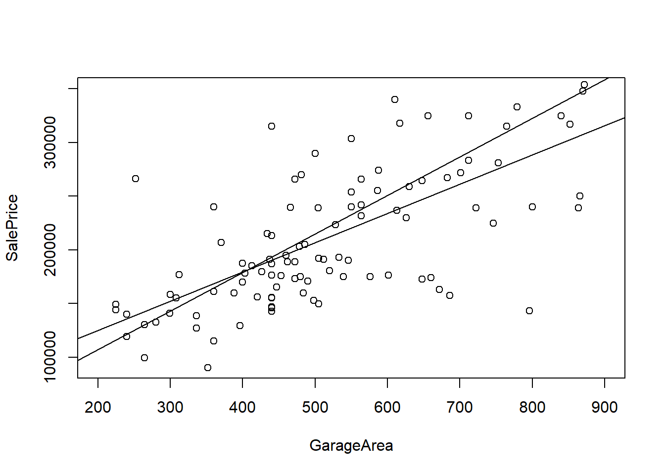
#plot(form, data = ,house_train)
mod<-lm(form, data = house_train)
#abline(mod)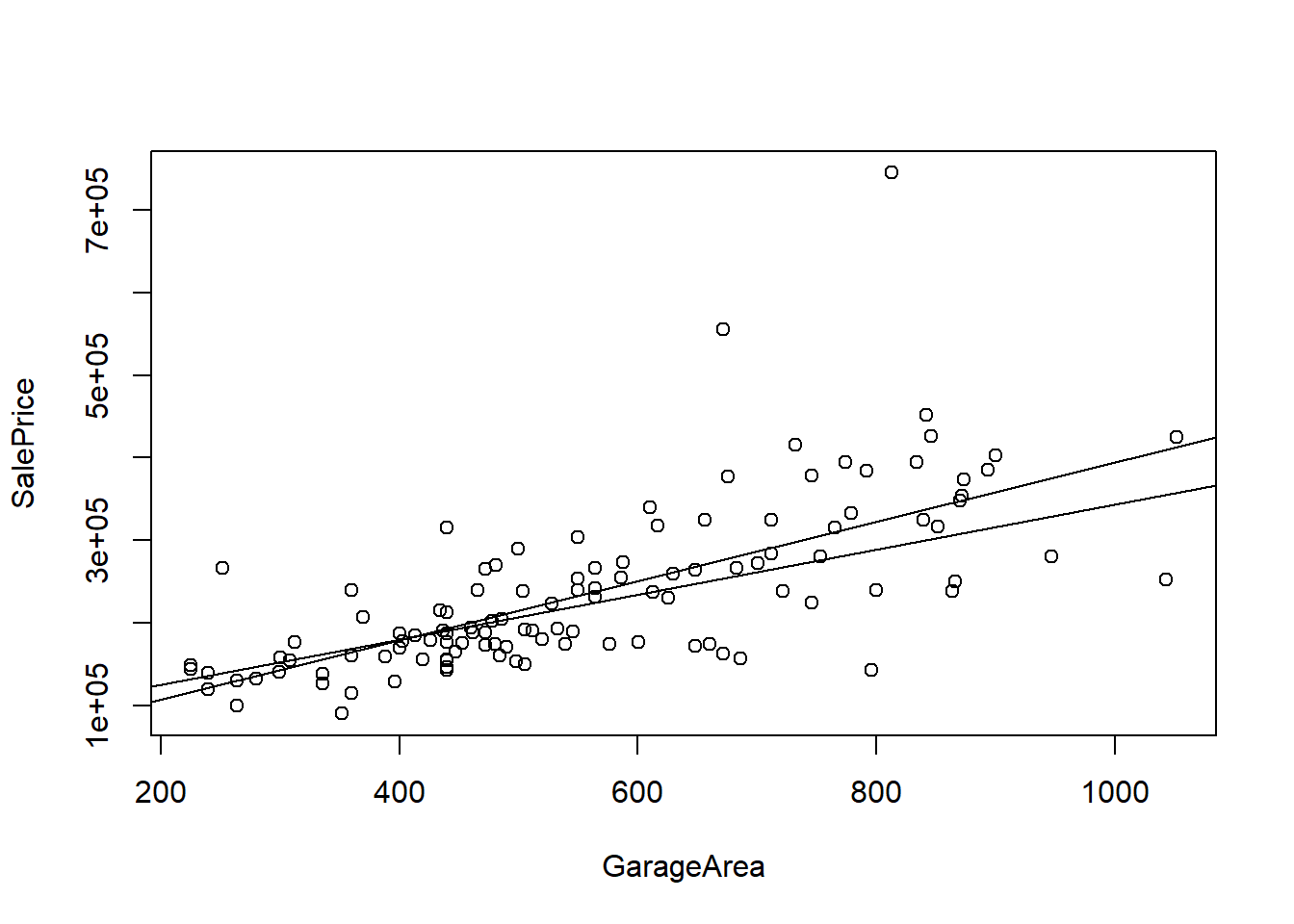
#indes<-"OverallQual"
#indes<-"YearRemodAdd"
indes<-"X2ndFlrSF"
#indes<-"GarageArea"
plot(house_train[,"SalePrice"],house_train[,indes])
abline(a = 500, b = 1)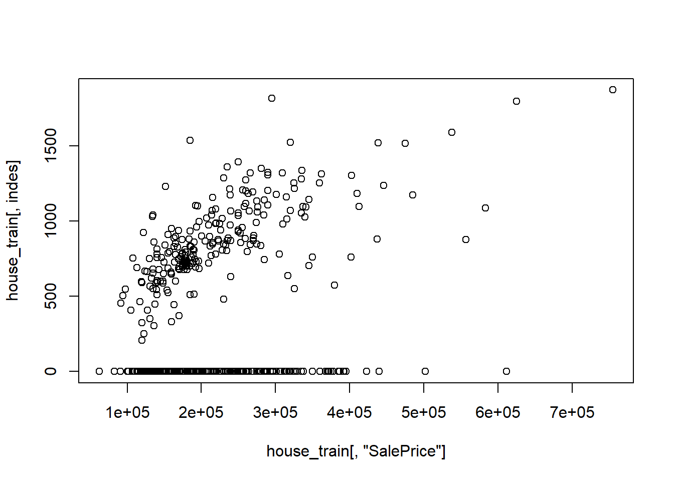
plot(house_test[,"SalePrice"],house_test[,indes])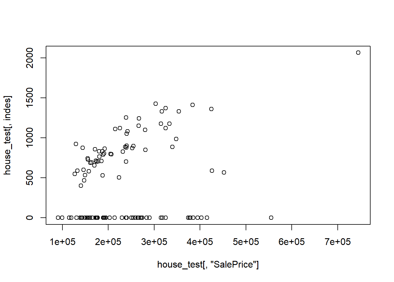
h_vars<-c("SalePrice",colnames(house_train[45:49]))

panel.cor <- function(x, y, digits = 2, prefix = "", cex.cor, ...)
{
    usr <- par("usr"); on.exit(par(usr))
    par(usr = c(0, 1, 0, 1))
    r <- abs(cor(x, y,use="pairwise.complete.obs"))
    txt <- format(c(r, 0.123456789), digits = digits)[1]
    txt <- paste0(prefix, txt)
    if(missing(cex.cor)) cex.cor <- 0.8/strwidth(txt)
    text(0.5, 0.5, txt, cex = cex.cor * r)
}
pairs(na.omit(house_train[,h_vars]),upper.panel=panel.cor)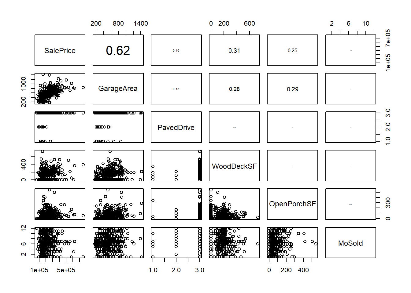
Models are frequently overfit when there are a small number of training samples relative to the flexibility or complexity of the model. Such a model is considered to have high variance or low bias.
A supervised model that is overfit will typically perform well on data the model was trained on, but perform poorly on data the model has not seen before (Krishnan 2020).
Underfitting occurs when the machine learning model does not capture variations in the data – where the variations in data are not caused by noise. Such a model is considered to have high bias, or low variance. A supervised model that is underfit will typically perform poorly on both data the model was trained on, and on data the model has not seen before. Examples of overfitting, underfitting, and a good balanced model (Krishnan 2020).
#knitr::include_graphics('images/overfit.jpg')2.1.8 Regularization models
Regularization is a method to balance overfitting and underfitting a model during training. Both overfitting and underfitting are problems that ultimately cause poor predictions on new data.
Regularization is a technique to adjust how closely a model is trained to fit historical data. One way to apply regularization is by adding a parameter that penalizes the loss function when the tuned model is overfit.
This allows use of regularization as a parameter that affects how closely the model is trained to fit historical data. More regularization prevents overfitting, while less regularization prevents underfitting. Balancing the regularization parameter helps find a good tradeoff between bias and variance.
summary(house[,"SalePrice"])
#>    Min. 1st Qu.  Median    Mean 3rd Qu.    Max.
#>   62383  159988  193690  222864  266625  755000
2.2 Appendix
2.2.1 Proof of \(E(MSE) =Var(\epsilon)+Var(\hat{y})+[Bias(\hat{y})]^2\)
\[E ((y-\hat{y})^2)=E((y-E(\hat{y})+E(\hat{y})-\hat{y})^2)=(y-E(\hat{y}))^2+E((E(\hat{y})-y)^2)+2E(y-E(\hat{y}))\ E(E(\hat{y})-\hat{y})\]
where
\[2E(y-E(\hat{y}))\ E(E(\hat{y})-\hat{y})=2E(y-E(\hat{y}))\ (E(\hat{y})-E(\hat{y}))=0\]
\[2E(y-E(\hat{y}))\ E(E(\hat{y})-\hat{y})=2E(y-E(\hat{y}))\ (E(\hat{y})-E(\hat{y}))=0\]