1 Python Basics | Machine learning introductory guide Python

1.1 1 Jupyter Notebook

In this book, we will work on Jupyter Notebook, which is the original web application for creating and sharing computational documents. It offers a simple, streamlined, document-centric experience.

See more about in https://jupyter.org/.

1.2 Data types, numerical and text objects

Python is a programming language that lets us work quickly and integrate systems more effectively and contains many data types as part of the core language (py?).

The entities that we can create and manipulate in Python are called objects. We could make those objects by applying the assignment operator (‘=’).

For example, we create the object “a”; winch has assigned the value 4.

x=4
x
#> 4

Each object in Python has tho characteristics, object type and object value.

Object type tells Python what kind of an object it’s dealing with. A type could be a number, a string, a list, or something else. In this book, we will use those types of objects. Also, we will cover more complex data structures such as dictionaries, arrays and data frames.

The function type() shows us the object type. For example, the object x is an integer(int):

type(x)
#> <class 'int'>

In this example, the object type is an integer(int), and the value is 4.

Besides integers, Python provides other numeric types, floating point numbers, and complex numbers (for example (5j). For example:

type(1.23)
#> <class 'float'>

An example of string (str) would be:

y="Apple"
type(y)
#> <class 'str'>

We are adding the ” ” to tell Python that Apple is a string.

1.3 List and object attributes

A list is another useful object in Python, a vector of integers, strings, or both.

liste=[1,2,3]
liste
#> [1, 2, 3]

type(liste)
#> <class 'list'>

Objects whose value can change are called mutable objects, whereas objects whose value is unchangeable after they’ve been created are called immutable.

4 # is inmutable

# but liste is mutable
#> 4
liste=["a","b"]

Most Python objects have either data or functions or both associated with them. These are known as attributes. The name of the attribute follows the name of the object. And these two are separated by a dot in between them. The two types of attributes are called either data attributes or methods.

The “list” data type has some more methods. Here are all of the methods of “list” objects:

s=[1,2,3,4]
dir(s)[1:10]
#> ['__class__', '__class_getitem__', '__contains__', '__delattr__', '__delitem__', '__dir__', '__doc__', '__eq__', '__format__']

We printed only the first ten methods. But in the list, you can find more methods. In this section, we will cover some examples—the method append, which appends an object to the end of the list.

s.append(6)
s
#> [1, 2, 3, 4, 6]

A data attribute contains information about the object. For example, to get the number of elements of a list, we use the data method “len.”

len(s)
#> 5

There are other ways to manipulate a “list” without a method. For instance, to concatenate two different lists:

t=[12,14,16]
s=s+t
s
#> [1, 2, 3, 4, 6, 12, 14, 16]

To select an element of a list, for example, selecting the second element of the list:

s[1]
#> 2

As you can see, instead of typing the s[2], we write the number one because Python starts counting to zero.

s[0]
#> 1

For example, replace the number 3 in lis “s” with the number 100 to replace an element of a list.

s[2]=100
s
#> [1, 2, 100, 4, 6, 12, 14, 16]

To remove an element, for example, number 2:

s.remove(2)
s
#> [1, 100, 4, 6, 12, 14, 16]

1.4 Dictionaries

Dictionaries are useful objects for performing fast look-ups on underscored data.

grades_dict={"Paulina": 100, "Coral":95} 
grades_dict
#> {'Paulina': 100, 'Coral': 95}

The “dictionaries” have two components, keys and values. The keys:

grades_dict.keys()
#> dict_keys(['Paulina', 'Coral'])

And values:

grades_dict.values()
#> dict_values([100, 95])

Dictionaries are mutable, then we can modify their content, by adding a new element:

grades_dict["Alejandra"]=120
grades_dict
#> {'Paulina': 100, 'Coral': 95, 'Alejandra': 120}

Or modifying an element:

# modify an element
grades_dict["Alejandra"]=grades_dict["Alejandra"]-30
grades_dict
#> {'Paulina': 100, 'Coral': 95, 'Alejandra': 90}

We could ask for an element in the dictionary:

# members

"Karina" in grades_dict
#> False

We could combine two or more lists into a dictionary, having two keys and four values each:

names=["Eugenio","Luis","Isa","Gisell"]
numbers=[9,17,80,79]
combine = {"Letthers":names,"Colors":numbers}
combine
#> {'Letthers': ['Eugenio', 'Luis', 'Isa', 'Gisell'], 'Colors': [9, 17, 80, 79]}

Or we may want to use one list for the keys and the other for the values:

stud= dict(zip(names, numbers))
stud
#> {'Eugenio': 9, 'Luis': 17, 'Isa': 80, 'Gisell': 79}

1.5 Python modules

Python also contains building functions that all Python programs can use. The user could make functions or could be developed by someone else in a library.

The Python modules are code libraries, and you can import Python modules using the import statements. Two of the most popular libraries in Python are Pandas and Numpy.

1.5.1 Pandas data frames

It is a Python package that provides fast, flexible, and expressive data structures designed to make working with “relational” or “labeled” data easy and intuitive. It is the fundamental high-level building block for practical, real-world data analysis in Python. Additionally, it aims to become the most powerful and flexible open-source data analysis/manipulation tool available in any language. It is already well on its way toward this goal.

We will use it to create and manipulate data frames, which are two-dimensional, size-mutable, potentially heterogeneous tabular data.

To install the Pandas module, we write in a notebook cell or in the Conda terminal prompt “pip install pandas” in the Terminal prompt.

pip install pandas

To import the library we use the “import” statement:

import pandas as pd

After the name Pandas, we use the “as” statement to give pandas a short name. Then, when we use it, it is easier to call pd than pandas. For example, to create a data frame, we have to call the “pd”. and the method DataFrame, referring to that we are calling the method DataFrame from the library pandas:

name=["Vale","Diana","Ivan","Vivi"]
df = pd.DataFrame(name,columns=["Column 1"])
df

	Column 1
0	Vale
1	Diana
2	Ivan
3	Vivi

In the previous example, an argument of the function is columns; winch is the column name of the data frame. To know more about the function and its arguments, we could ask like this:

help(pd.DataFrame) # or like this: pd.DataFrame?

In the previous example, by default, the index, the left column without a title, is numbered from zero to 3, but if we want to change the index:

name=["Vale","Diana","Ivan","Vivi"]
numbers=[51,11,511,50]
df = pd.DataFrame(name,columns=["Column 1"],index=numbers)
df

	Column 1
51	Vale
11	Diana
511	Ivan
50	Vivi

We could take advantage of the creation of a dictionary and transform it into a data frame:

my_dict=dict(zip(name, numbers))
sn=pd.DataFrame(my_dict,index=["Student_number"])
sn

	Vale	Diana	Ivan	Vivi
Student_number	51	11	511	50

If we want to have the student_number as columns instead of a row, we could transpose the data frame:

sn.transpose()

	Student_number
Vale	51
Diana	11
Ivan	511
Vivi	50

name=["Estefanía","Laura Yanet","María Guadalupe","Karla Lizette"]
nick=["Estef","Yanet","Lupita","Karla"]
number=[1,2,3,4]

# We use two list to create the dictionary
combine = {"Nick_name":nick,"Name":name}

# and from the dictionary we create the  data frame
df=pd.DataFrame(combine,index=number)
df

	Nick_name	name
1	Estef	Estefanía
2	Yanet	Laura Yanet
3	Lupita	María Guadalupe
4	Karla	Karla Lizette

To apply a method (function) to the data frame, we must type the Pandas object and a dot before the method. A useful method is “shape,” which gives us the number of rows and columns.

df.shape 
#> (4, 2)

To rename a data frame column:

df=df.rename(columns={"Nick_name": "Nick", "name": "Names"})
df

	Nick	Names
1	Estef	Estefanía
2	Yanet	Laura Yanet
3	Lupita	María Guadalupe
4	Karla	Karla Lizette

It also applies for index:

df=df.rename(index={1: "x", 2: "y", 3: "z",4:"w"})
df

	Nick	Names
x	Estef	Estefanía
y	Yanet	Laura Yanet
z	Lupita	María Guadalupe
w	Karla	Karla Lizette

1.5.2 Selecting rows and columns in a data frame

To select a column, we could type the column name:

df["Nick"]
#> x     Estef
#> y     Yanet
#> z    Lupita
#> w     Karla
#> Name: Nick, dtype: object

The resulting object is a pandas series, a one-dimensional object, such as a list, but with an index, in this case, the data frame index.

type(df["Nick"])
#> <class 'pandas.core.series.Series'>

If we want to keep the data frame type, we should add the square brackets twice:

df[["Nick"]]

	Nick
x	Estef
y	Yanet
z	Lupita
w	Karla

Or two columns at once:

df[["Nick","Names"]]

	Nick	Names
x	Estef	Estefanía
y	Yanet	Laura Yanet
z	Lupita	María Guadalupe
w	Karla	Karla Lizette

To select rows, we use the method “.loc”.

df.loc[["y"]]

	Nick	Names
y	Yanet	Laura Yanet

df.loc[["y","z"]]

	Nick	Names
y	Yanet	Laura Yanet
z	Lupita	María Guadalupe

The “loc” method also works for selecting a column:

df.loc[:, ("Nick","Names")]

Or more than one column:

	Nick	Names
x	Estef	Estefanía
y	Yanet	Laura Yanet
z	Lupita	María Guadalupe
w	Karla	Karla Lizette

Sometimes is useful to select by position. We use the method .iloc[ rows, columns ] in this case. For example, to select the second and third columns:

df.iloc[: , 1:]

	Names
x	Estefanía
y	Laura Yanet
z	María Guadalupe
w	Karla Lizette

The left side of the comma is for selecting rows, and the right is for columns. Another example:

df.iloc[: , 0:2]

	Nick	Names
x	Estef	Estefanía
y	Yanet	Laura Yanet
z	Lupita	María Guadalupe
w	Karla	Karla Lizette

For rows:

df.iloc[2: , ]

	Nick	Names
z	Lupita	María Guadalupe
w	Karla	Karla Lizette

To insert a new column:

num_2=list(range(4))

df["Numbers_2"]=num_2
df

	Nick	Names	Numbers_2
x	Estef	Estefanía	0
y	Yanet	Laura Yanet	1
z	Lupita	María Guadalupe	2
w	Karla	Karla Lizette	3

The range method return an object that produces a sequence of integers from start (inclusive) to stop (exclusive) by step. range(i, j) produces i, i+1, i+2, …, j-1.

To drooping colum(s):

df.drop(columns=['Names'])

	Nick	Numbers_2
x	Estef	0
y	Yanet	1
z	Lupita	2
w	Karla	3

df.drop(columns=['Names',"Numbers_2"])

	Nick
x	Estef
y	Yanet
z	Lupita
w	Karla

1.6 Reading Excel and csv files

You can download the Excel file by copying and pasting and pasting to a browser through the following link:

https://github.com/abernal30/ML_python/blob/main/df.xlsx

I stored the file in a sub-directory named “data,” and I called “df.xlsx”

To verify the names of the Sheets, we use the following code:

import pandas as pd
sheets=pd.ExcelFile("data/df.xlsx").sheet_names
sheets
#> ['Sheet1', 'Sheet2', 'Sheet3']

I use the function read_excel of the Pandas library to read the Excel file. In this case, I use the argument sheet_name=sheets[0], equivalent to sheet_name=“Sheet1”.

data=pd.read_excel("data/df.xlsx",sheet_name=sheets[0])
data

	Unnamed: 0	Unnamed: 1	Unnamed: 2	Unnamed: 3
0	nan	Título HOJA 1	nan	nan
1	nan	nan	X	Y
2	A	nan	2	10
3	B	nan	50	nan
4	C	nan	nan	25
5	nan	nan	nan	nan
6	D	nan	20	34
7	E	nan	200	23

Sometimes is useful to read the Excel file and define as the index a column of the Excel file. In this case, we want the column “Unnamed: 0”.

data=pd.read_excel("data/df.xlsx",sheet_name=sheets[0],index_col="Unnamed: 0")
data

	Unnamed: 1	Unnamed: 2	Unnamed: 3
nan	Título HOJA 1	nan	nan
nan	nan	X	Y
A	nan	2	10
B	nan	50	nan
C	nan	nan	25
nan	nan	nan	nan
D	nan	20	34
E	nan	200	23

1.7 Numpy modules

NumPy is the fundamental package for scientific computing in Python. It is a Python library that provides a multidimensional array object, various derived objects (such as masked arrays and matrices), and an assortment of routines for fast operations on arrays, including mathematical, logical, shape manipulation, sorting, selecting, I/O, discrete Fourier transforms, basic linear algebra, basic statistical operations, random simulation and much more.

In machine learning models is useful to work with Numpy arrays. NumPy’s main object is the homogeneous multidimensional array. For example, we could define variables x and y as an array.

import numpy as np

X=np.array([[1,2,3],[4,5,6]])
X
#> array([[1, 2, 3],
#>        [4, 5, 6]])

Or we can create a matrix for several variables.

Y=np.array([[2,4,6],[8,10,12]])
Y
#> array([[ 2,  4,  6],
#>        [ 8, 10, 12]])

Sometimes is useful to simulate a missing value:

np.nan
#> nan

1.8 Missing value management

Suppose we read the Excel we used in the section “Reading Excel and CSV files.” We want to work with the “Unnamed: 2” column, as a header we use the second row.

data=pd.read_excel("data/df.xlsx",sheet_name="Sheet1",index_col="Unnamed: 0",header=2)
data

	Unnamed: 1	X	Y
A	nan	2.000000	10.000000
B	nan	50.000000	nan
C	nan	nan	25.000000
nan	nan	nan	nan
D	nan	20.000000	34.000000
E	nan	200.000000	23.000000

To get a better look at our data frame, we select the second and third columns, with the following method:

data=data.iloc[:,1:]
data

	X	Y
A	2.000000	10.000000
B	50.000000	nan
C	nan	25.000000
nan	nan	nan
D	20.000000	34.000000
E	200.000000	23.000000

A first look to detect missing values is using the following function:

data.isna().sum()
#> X    2
#> Y    2
#> dtype: int64

It tells us that both columns, “X” and “Y”, have two missing values.

We have many alternatives to manage them. First eliminating the row that has at least one missing value.

data.dropna()

	X	Y
A	2.000000	10.000000
D	20.000000	34.000000
E	200.000000	23.000000

Another alternative is filling them with a value, for example the last value available in the data frame.

data.fillna(method='ffill')

	X	Y
A	2.000000	10.000000
B	50.000000	10.000000
C	50.000000	25.000000
nan	50.000000	25.000000
D	20.000000	34.000000
E	200.000000	23.000000

Or with a value such as zero:

data_clenan=data.replace(np.nan,0)

# which is equivalent to 
#data.fillna(0)

data_clenan

	X	Y
A	2.000000	10.000000
B	50.000000	0.000000
C	0.000000	25.000000
nan	0.000000	0.000000
D	20.000000	34.000000
E	200.000000	23.000000

We still have a missing value in the index, after letter “C”. The next function

# This function skips the index elements of a data frame that are missing values, space or: ".",",",";",";","'",'""'.
# It returns a data frame without the ignored elements.
# Parameters:
# df: data frame. The object for which the method is called

#---- Do not change anything from here ----
def clean_na_index2(df):
    skips=[".",",",";",";","'",'""'," ",np.nan]
    con=[name_ind for name_ind in df.index if name_ind not in skips]
    return  df.loc[con, ]
#----- To here ------------

#Run the code so that Python can execute the function

df_index_clean=clean_na_index2(data_clean)
df_index_clean

	X	Y
A	2.000000	10.000000
B	50.000000	0.000000
C	0.000000	25.000000
D	20.000000	34.000000
E	200.000000	23.000000

1.9 Merge, joint or concatenate data frames

Suppose we want to merge the object df_index_clean of the previous section, with the data frame in the “Sheet2” of the Excel file “df.xlsx”:

#,header=2
data=pd.read_excel("data/df.xlsx",sheet_name="Sheet2",index_col="Unnamed: 0")
data

	W	Z
A	2	10
B	50	30
C	30	25
D	20	34
E	200	23

In this case, both data frames have the same index:

print(data.index)
#> Index(['A', 'B', 'C', 'D', 'E'], dtype='object')
print(df_index_clean.index)
#> Index(['A', 'B', 'C', 'D', 'E'], dtype='object')

Then we can use the function concat. The argument axis=1 is to concatenate the columns of both data frames in the columns.

pd.concat([df_index_clean,data],axis=1)

	X	Y	W	Z
A	2.000000	10.000000	2	10
B	50.000000	0.000000	50	30
C	0.000000	25.000000	30	25
D	20.000000	34.000000	20	34
E	200.000000	23.000000	200	23

Otherwise it would concatenate in the index (rows)

pd.concat([df_index_clean,data])

	X	Y	W	Z
A	2.000000	10.000000	nan	nan
B	50.000000	0.000000	nan	nan
C	0.000000	25.000000	nan	nan
D	20.000000	34.000000	nan	nan
E	200.000000	23.000000	nan	nan
A	nan	nan	2.000000	10.000000
B	nan	nan	50.000000	30.000000
C	nan	nan	30.000000	25.000000
D	nan	nan	20.000000	34.000000
E	nan	nan	200.000000	23.000000

1.10 API´s (Application Programming Interface)

1.10.1 The “yfinance” library

It was designed to download market data from Yahoo! Finance. To see how to install it and more information: https://pypi.org/project/yfinance/

import yfinance as yf

msft = yf.Ticker("MSFT")

The following code shows a dictionary that contains information such as company address, business summary, etc.

msft.info

To download the ticker´s prices.

msft.history(period="1mo").head()

	Open	High	Low	Close	Volume	Dividends	Stock Splits
Date
2023-05-01 00:00:00-04:00	306.300422	307.926871	304.484384	304.893494	21294100	0.000000	0.000000
2023-05-02 00:00:00-04:00	307.088685	308.505570	303.247077	304.743805	26404400	0.000000	0.000000
2023-05-03 00:00:00-04:00	305.951182	307.936831	303.426702	303.736023	22360800	0.000000	0.000000
2023-05-04 00:00:00-04:00	305.571981	307.088685	302.738180	304.743805	22519900	0.000000	0.000000
2023-05-05 00:00:00-04:00	305.053143	311.289510	303.606293	309.972382	28181200	0.000000	0.000000

As you can see in the method help (help(msft.history)), valid periods are: 1d,5d,1mo,3mo,6mo,1y,2y,5y,10y,ytd,max

Also there are other parameters such as interval=‘1d’: intervals: 1m,2m,5m,15m,30m,60m,90m,1h,1d,5d,1wk,1mo,3mo

For some of the procedures we will apply in this book, we require the dates in a format, for example “%Y-%m-%d”. And the

import yfinance as yf
# This function download market data from Yahoo! Finance's
# It returns a data frame with a specific format date. 
# Parameters:
# ticker: Yahoo finance ticker symbol
# per: valid periods are: 1d,5d,1mo,3mo,6mo,1y,2y,5y,10y,ytd,max
# inter: intervals: 1m,2m,5m,15m,30m,60m,90m,1h,1d,5d,1wk,1mo,3mo
# price_type: Open', 'High', 'Low', 'Close', 'Volume', 'Dividends', 'Stock Splits
# format_date:  index format date
# d_ini: initial date if the subset
# d_fin: final date of the subset

#---- Do not change anything from here ----
def my_yahoo(ticker,per,inter,price_type,format_date,d_ini,d_fin):
    import pandas as pd
    x = yf.Ticker(ticker)
    hist = x.history(period=per,interval=inter)
    date=list(hist.index)
    hist_date=[date.strftime(format_date) for date in date]
    price=list(hist[price_type])
    hist={ticker:price}
    hist=pd.DataFrame(hist,index=hist_date)
    return hist.loc[d_ini:d_fin]
#----- To here ------------

#Run the code cell so that Python can execute the function

format_date="%Y-%m-%d"
per="5y"
inter='1mo'
price_type="Close"
ticker="^MXX"
d_ini="2021-01-01"
d_fin="2022-12-01"

ipc=my_yahoo(ticker,per,inter,price_type,format_date,d_ini,d_fin)
ipc.head()

	^MXX
2021-01-01	42985.730469
2021-02-01	44592.910156
2021-03-01	47246.261719
2021-04-01	48009.718750
2021-05-01	50885.949219

1.10.2 Banxico API

To download historical information of the Mexican central bank (BANXICO). Such as interest rates, exchange rates and other macroeconomic information. To see how to install it and more information: https://pypi.org/project/sie-banxico/

We need to get a token in the following web page: https://www.banxico.org.mx/SieAPIRest/service/v1/token?locale=en

The token must look like this. And you have to store it in an object, for example:

token = "e3980208bf01ec653aba9aee3c2d6f70f6ae8b066d2545e379b9e0ef92e9de25"

In the same web page you could see the Series catalog, which are the variable ID:

from sie_banxico import SIEBanxico

# This function download information from BANXICO 
# It returns a data frame with a specific format date
# Parameters:
# token: The token object
# my_series: Banxico´s Series ID´s
# my_series_name: The short name we want to assign to the Serie.
# d_in: initian date of the subset
# d_fin: final date of the subset
# format_date: index format date

#---- Do not change anything from here ----
def my_banxico_py(token,my_series,my_series_name,d_in,d_fin,format_date):
    import pandas as pd
    le=len(my_series)
    ser=0
    if(le==1):
        ser=0
        api = SIEBanxico(token = token, id_series = my_series[ser])
        timeseries_range=api.get_timeseries_range(init_date=d_in,end_date=d_fin)
        timeseries_range=timeseries_range['bmx']['series'][0]['datos']
        data=pd.DataFrame(timeseries_range)
        dates=[pd.Timestamp(date).strftime(format_date) for date in list(data["fecha"])]
        data=pd.DataFrame({my_series_name[ser]:list(data["dato"])},index=dates)
    else:
        ser=0
        api = SIEBanxico(token = token, id_series = my_series[ser])
        timeseries_range=api.get_timeseries_range(init_date=d_in, end_date=d_fin)
        timeseries_range=timeseries_range['bmx']['series'][0]['datos']
        data=pd.DataFrame(timeseries_range)
        dates=[pd.Timestamp(date).strftime(format_date) for date in list(data["fecha"])]
        data=pd.DataFrame({my_series_name[ser]:list(data["dato"])},index=dates)
        for ser in range(1,le):
            api = SIEBanxico(token = token, id_series = my_series[ser])
            timeseries_range=api.get_timeseries_range(init_date=d_in, end_date=d_fin)
            timeseries_range=timeseries_range['bmx']['series'][0]['datos']
            data2=pd.DataFrame(timeseries_range)
            dates2=[pd.Timestamp(date).strftime(format_date) for date in list(data2["fecha"])]
            data2=pd.DataFrame({my_series_name[ser]:list(data2["dato"])},index=dates2)
            data=pd.concat([data,data2],axis=1)
    ban_names=list(data.columns)
    for col_i in range(data.shape[1]):
        cel_num=[float(cel) for cel in data[ban_names[col_i]]]
        data[ban_names[col_i]]=cel_num
    return data
  
#----- To here ------------

For this example, we want to download the following Series:

SF17908: Exchange rate Pesos per US dollar

SF282: 28 days Mexican treasury bills

SP74660: Mexican inflation rate

SR16734: Global indicator of Mexican economic activity

#Run the code cell so that Python can execute the function
my_series=['SF17908' ,'SF282',"SP74660","SR16734"]
my_series_name=["TC","Cetes_28","Mex_inflation","igae"]
d_in='2021-01-01'
d_fin='2022-12-01'
format_date="%Y-%d-%m"
my_banxico_py(token,my_series,my_series_name,d_in,d_fin,format_date).head()

	TC	Cetes_28	Mex_inflation	igae
2021-01-01	19.921500	4.220000	0.360000	105.545700
2021-02-01	20.309700	4.120000	0.390000	102.802900
2021-03-01	20.755500	4.050000	0.540000	111.518600
2021-04-01	20.015300	4.070000	0.370000	107.834900
2021-05-01	19.963100	4.060000	0.530000	111.176800

1.11 Plots or graphs

For example, we use the method plot to plot the APPLE historical price. First, we download the prices.

format_date="%Y-%m-%d"
per="5y"
inter='1mo'
price_type="Close"
ticker="AAPL"
d_ini="2023-01-01"
d_fin="2023-05-01"
apple=my_yahoo(ticker,per,inter,price_type,format_date,d_ini,d_fin)

Then we use the function plot;

apple.plot(title="APPLE close price", ylabel="Price in $",xlabel="Date");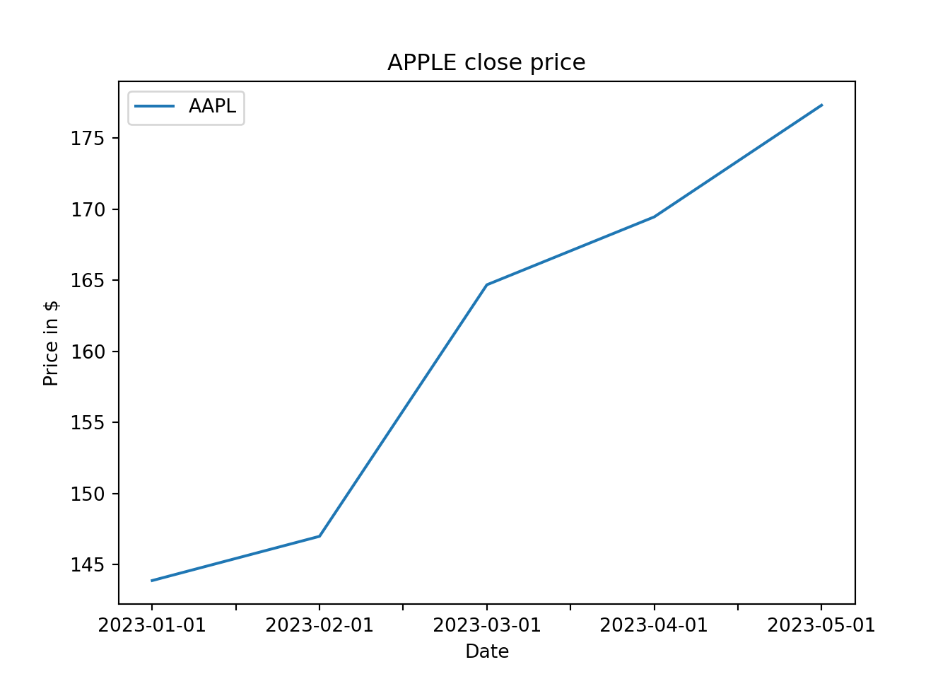

1.12 Dates management

In this section we mange the data frame dates.

data=pd.read_excel("data/df.xlsx",sheet_name="Sheet3")
#,index_col="Unnamed: 0"
data

	date	Sales
0	Ene 2021	5
1	Feb 2021	7
2	Mar 2021	60
3	Abr 2021	20
4	May 2021	21

For some analysis in machine learning, we require to have the index data as date format. The previous data frame index type is a string:

type(data.index[0])
#> <class 'int'>

Then, we use the following function:

# This function transforms the data frame index into a date format  
# (Timestamp). 
# It returns a data frame with the new date index
# Parameters:
# data: data frame with two columns, a date column and another one
# i_date: is the start date of the new index
# freq_i; frequency if the new index, "y" for year, "m" month, "d" day, "h" hour.
# col_name: name of the column in the data frame data that is not the date
# date_name= name of the column in the data that is the date
#---- Do not change anything from here ----
def index_date(data,i_date,freq_i,col_name,date_name):
  dat=data.set_index(date_name)
  ventas_s= pd.Series(
  list(dat[col_name]), index=pd.date_range(i_date, periods=len(dat),
  freq=freq_i), name=col_name)
  return pd.DataFrame(ventas_s)
#----- To here ------------

#Run the code so that Python can execute the function

i_date="1-1-2020"
freq_i="m"
col_name="Sales"
date_name="date"
data_ind_date=index_date(data,i_date,freq_i,col_name,date_name)
data_ind_date

Now the index is in a “Timestamp” format. For the moment, let’s say that it is a date format.

	Sales
2020-01-31 00:00:00	5
2020-02-29 00:00:00	7
2020-03-31 00:00:00	60
2020-04-30 00:00:00	20
2020-05-31 00:00:00	21