5  Portfolio management

import pandas as pd
import numpy as np
import matplotlib.pyplot as plt

In this section we use the filtered stocks of the previous chapter to build a Markowitz portfolio (Markowitz 1952). First we will apply the example for a two stock portfolio. Then, we extend the analysis for all the stocks.

data=pd.read_csv("https://raw.githubusercontent.com/abernal30/AFP_py/refs/heads/main/data/portfolio.csv",index_col=0) # en caso de no haber realizado el ejercicio de la seción anterior
data.head()

	ABT.Close	BAC.PE.Close	C.PJ.Close	NVS.Close	UNH.Close	WFC.PL.Close	CSCO.Close	JPM.PD.Close	WFC.PQ.Close	MCD.Close	...	BML.PG.Close	TCTZF.Close	TCEHY.Close	CVX.Close	SHEL.Close	AVGO.Close	INTC.Close	NVSEF.Close	ADBE.Close	TMUS.Close
date
01/02/2020	86.949997	24.511700	28.570000	94.949997	292.500000	1452.510010	48.419998	27.639999	27.629999	200.789993	...	21.480000	49.880001	49.880001	121.430000	59.740002	322.390015	60.840000	94.800003	334.429993	78.589996
01/03/2020	85.889999	24.600000	28.719999	94.790001	289.540009	1457.000000	47.630001	27.660000	27.780001	200.080002	...	21.420000	48.930000	49.029999	121.010002	60.209999	314.190002	60.099998	93.250000	331.809998	78.169998
01/06/2020	86.339996	24.497101	28.719999	95.430000	291.549988	1467.469971	47.799999	27.580000	27.690001	202.330002	...	21.469999	48.700001	48.770000	120.599998	60.959999	313.720001	59.930000	94.349998	333.709991	78.620003
01/07/2020	85.860001	24.510000	28.629999	94.480003	289.790009	1473.500000	47.490002	27.500000	27.500000	202.630005	...	21.429300	49.770000	49.779999	119.059998	60.400002	312.640015	58.930000	95.000000	333.390015	78.919998
01/08/2020	86.209999	24.440001	28.709999	94.480003	295.899994	1480.000000	47.520000	27.549999	27.559999	205.910004	...	21.930000	49.650002	49.650002	117.699997	59.689999	308.739990	58.970001	94.720001	337.869995	79.419998

5 rows × 34 columns

The prices returns.

ret_all=data.pct_change()
ret_all.head()

	ABT.Close	BAC.PE.Close	C.PJ.Close	NVS.Close	UNH.Close	WFC.PL.Close	CSCO.Close	JPM.PD.Close	WFC.PQ.Close	MCD.Close	...	BML.PG.Close	TCTZF.Close	TCEHY.Close	CVX.Close	SHEL.Close	AVGO.Close	INTC.Close	NVSEF.Close	ADBE.Close	TMUS.Close
date
01/02/2020	NaN	NaN	NaN	NaN	NaN	NaN	NaN	NaN	NaN	NaN	...	NaN	NaN	NaN	NaN	NaN	NaN	NaN	NaN	NaN	NaN
01/03/2020	-0.012191	0.003602	0.005250	-0.001685	-0.010120	0.003091	-0.016316	0.000724	0.005429	-0.003536	...	-0.002793	-0.019046	-0.017041	-0.003459	0.007867	-0.025435	-0.012163	-0.016350	-0.007834	-0.005344
01/06/2020	0.005239	-0.004183	0.000000	0.006752	0.006942	0.007186	0.003569	-0.002892	-0.003240	0.011246	...	0.002334	-0.004701	-0.005303	-0.003388	0.012456	-0.001496	-0.002829	0.011796	0.005726	0.005757
01/07/2020	-0.005559	0.000527	-0.003134	-0.009955	-0.006037	0.004109	-0.006485	-0.002901	-0.006862	0.001483	...	-0.001896	0.021971	0.020709	-0.012769	-0.009186	-0.003443	-0.016686	0.006889	-0.000959	0.003816
01/08/2020	0.004076	-0.002856	0.002794	0.000000	0.021084	0.004411	0.000632	0.001818	0.002182	0.016187	...	0.023365	-0.002411	-0.002611	-0.011423	-0.011755	-0.012474	0.000679	-0.002947	0.013438	0.006336

5 rows × 34 columns

5.1 Portfolio of two stocks

We will estimate the return, standard deviation and Sharpe ratio for a portfolio of two stocks. And also making an aleatory weight.

ret_two=ret_all.loc[:,("CMCSA.Close","TMUS.Close")]
ret_two.head()

	CMCSA.Close	TMUS.Close
date
01/02/2020	NaN	NaN
01/03/2020	-0.007935	-0.005344
01/06/2020	-0.007554	0.005757
01/07/2020	0.005821	0.003816
01/08/2020	0.010238	0.006336

We know that the arithmetic mean portfolio return for two assets

\[r_{p}= w_{A}*r_{A}+w_{B}*r_{B}\]

Where - \(r_{p}\) is the portfolio return - \(w_{A}, w_{B}\) are the weight of the asset A, B respectively - \(r_{A},r_{B}\) are the returns of the asset A, B respectively

The expected return (mean) for two assets:

ret_two.mean()

CMCSA.Close    0.000147
TMUS.Close     0.001091
dtype: float64

Now we create the portfolio random weights

np.random.seed(1) # To get the same random number, the number 1, it is because Python has many predefined random numbers.

ran=np.random.rand(2) #the simulation of two random numbers, the two, is because we require two random numbers


# The following is so that it always adds up to 100% or 1
su=np.sum(ran) #

we=ran/su # this are the weights
we

array([0.36666223, 0.63333777])

To review that the sum is 100% or 1.00

sum(we)

1.0

We first estimate the portfolio return manually

0.000147*0.36666223+0.001091*0.63333777 

0.00074487085488

Now we estimate the portfolio return with a Python function, which apply for two or more assets.

rend_d=np.sum(ret_two.mean()*we) 
rend_d

0.0007447264667679712

To estimate the annualized return

rend_a=(1+rend_d)**252-1 
rend_a

0.20635235323618217

Portfolio variance for two assets

\[\sigma_{p}^2= w_{A}^2*\sigma_{A}^2+w_{B}^2*\sigma_{B}^2+ 2 * cov(r_{A},r_{B})w_{A}*w_{B}\]

Where: - \(\sigma_{p}^2\) is the portfolio variance - \(w_{A}, w_{B}\) are the weigth of the asset A, B respectively - \(\sigma_{A}^2, \sigma_{B}^2\) are the variance of asset A, B respectively - \(cov(r_{A},r_{B})\) is the covariance of the return of the asset A and B

Covariance matrix of the returns

cov=ret_two.cov()
cov

	CMCSA.Close	TMUS.Close
CMCSA.Close	0.000386	0.000237
TMUS.Close	0.000237	0.000451

This is the daily portfolio variance mannually

0.000386*pow(0.36666223,2)+0.000451*pow(0.63333777,2)+2*0.000237*0.36666223*0.63333777

0.00034287071785981196

This is the daily portfolio variance using Python formulas, which apply for two or more assets.

varp_day=np.dot(np.dot(we,cov),we.T)
varp_day

0.0003429252889213939

This is the annual portfolio standard deviation using Python formulas, which apply for two or more assets.

desvp_a=np.sqrt(varp_day)*np.sqrt(252)
desvp_a

0.2939679792225529

The Shape ratio

\[Shape\ ratio=\frac{portfolio\ return - risk\ free\ rate}{portfolio\ standard\ deviation} \]

r=0 # risk free 
sharpe=(rend_a-r)/desvp_a
sharpe 

0.7019552053999731

5.2 Portfolio of many assets

Here we get together the code of the previous section to do a Loop For for doing the same procedure for all the stocks inside the data frame ret_all.

retp=[]
sdp=[]
sharp=[]
wep=[]
n=10000 # number de simulations
r=0
for i in range(n):
 
  ran=np.random.rand(ret_all.shape[1]) 
  su=np.sum(ran)
  we=ran/su
  rend_d=np.sum(ret_all.mean()*we) 
  rend_a=(1+rend_d)**252-1
  cov=ret_all.cov() 
  varp_day=np.dot(np.dot(we,cov),we.T)
  desvp_a=np.sqrt(varp_day)*np.sqrt(252)
  sharpe=(rend_a-r)/desvp_a
  retp.append(rend_a) 
  sdp.append(desvp_a)
  sharp.append(sharpe) 
  wep.append(we) 

Also, we create a data frame with the result, the name of the portfolio standard deviation must be Stdev and Sharpe ratio Sharpe

metrics=pd.DataFrame({"Return":retp,"Stdev":sdp,"Sharpe":sharp})
metrics.head()

	Return	Stdev	Sharpe
0	0.082503	0.211402	0.390267
1	0.085297	0.199864	0.426775
2	0.087777	0.203849	0.430599
3	0.069707	0.199730	0.349008
4	0.088389	0.201766	0.438078

And a data frame with the weights.

weights_df=pd.DataFrame(wep,columns=ret_all.columns)
weights_df.head()

	ABT.Close	BAC.PE.Close	C.PJ.Close	NVS.Close	UNH.Close	WFC.PL.Close	CSCO.Close	JPM.PD.Close	WFC.PQ.Close	MCD.Close	...	BML.PG.Close	TCTZF.Close	TCEHY.Close	CVX.Close	SHEL.Close	AVGO.Close	INTC.Close	NVSEF.Close	ADBE.Close	TMUS.Close
0	0.000008	0.020231	0.009820	0.006179	0.012464	0.023124	0.026550	0.036056	0.028051	0.045853	...	0.005691	0.002613	0.011364	0.058762	0.006581	0.028179	0.064099	0.035678	0.046298	0.021113
1	0.043126	0.052432	0.001149	0.047125	0.062121	0.047000	0.017618	0.049583	0.006485	0.028137	...	0.006429	0.026011	0.043623	0.026019	0.003138	0.033665	0.041700	0.032346	0.059340	0.036848
2	0.048349	0.007357	0.007454	0.043211	0.021283	0.008850	0.049639	0.018612	0.040183	0.038854	...	0.021843	0.012685	0.048348	0.030703	0.000154	0.033029	0.017482	0.028207	0.047414	0.019121
3	0.052457	0.035991	0.000913	0.053664	0.039891	0.057583	0.009951	0.007918	0.053846	0.040233	...	0.007169	0.016119	0.033820	0.055982	0.032393	0.001077	0.046227	0.013451	0.046600	0.022394
4	0.057787	0.049996	0.037223	0.009131	0.004010	0.008120	0.002981	0.007193	0.015104	0.047712	...	0.041487	0.055474	0.010492	0.001243	0.004686	0.032546	0.040575	0.038067	0.021237	0.066157

5 rows × 34 columns

We can prove that the sum of each row, which represents the weights for each stock for a simulation, is one.

weights_df.iloc[0,].sum()

1.0

We concatenate the data frame with the metrics with the data frame with the weights.

port=pd.concat([metrics,weights_df],axis=1)
port.head()

	Return	Stdev	Sharpe	ABT.Close	BAC.PE.Close	C.PJ.Close	NVS.Close	UNH.Close	WFC.PL.Close	CSCO.Close	...	BML.PG.Close	TCTZF.Close	TCEHY.Close	CVX.Close	SHEL.Close	AVGO.Close	INTC.Close	NVSEF.Close	ADBE.Close	TMUS.Close
0	0.082503	0.211402	0.390267	0.000008	0.020231	0.009820	0.006179	0.012464	0.023124	0.026550	...	0.005691	0.002613	0.011364	0.058762	0.006581	0.028179	0.064099	0.035678	0.046298	0.021113
1	0.085297	0.199864	0.426775	0.043126	0.052432	0.001149	0.047125	0.062121	0.047000	0.017618	...	0.006429	0.026011	0.043623	0.026019	0.003138	0.033665	0.041700	0.032346	0.059340	0.036848
2	0.087777	0.203849	0.430599	0.048349	0.007357	0.007454	0.043211	0.021283	0.008850	0.049639	...	0.021843	0.012685	0.048348	0.030703	0.000154	0.033029	0.017482	0.028207	0.047414	0.019121
3	0.069707	0.199730	0.349008	0.052457	0.035991	0.000913	0.053664	0.039891	0.057583	0.009951	...	0.007169	0.016119	0.033820	0.055982	0.032393	0.001077	0.046227	0.013451	0.046600	0.022394
4	0.088389	0.201766	0.438078	0.057787	0.049996	0.037223	0.009131	0.004010	0.008120	0.002981	...	0.041487	0.055474	0.010492	0.001243	0.004686	0.032546	0.040575	0.038067	0.021237	0.066157

5 rows × 37 columns

Sort the values to wet the maximum Sharpe

port.sort_values(by="Sharpe",ascending=False).head()

	Return	Stdev	Sharpe	ABT.Close	BAC.PE.Close	C.PJ.Close	NVS.Close	UNH.Close	WFC.PL.Close	CSCO.Close	...	BML.PG.Close	TCTZF.Close	TCEHY.Close	CVX.Close	SHEL.Close	AVGO.Close	INTC.Close	NVSEF.Close	ADBE.Close	TMUS.Close
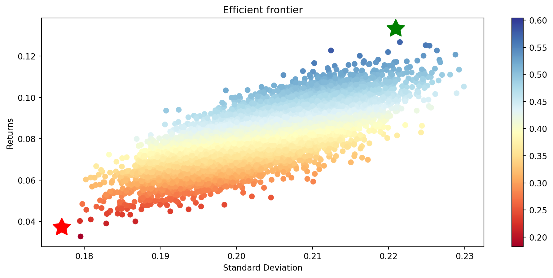
2194	0.133390	0.220914	0.603808	0.060100	0.026012	0.000724	0.016092	0.065260	0.013263	0.000725	...	0.024553	0.059973	0.024080	0.048028	0.028587	0.039303	0.001541	0.035531	0.060852	0.054208
5105	0.122734	0.212432	0.577759	0.023532	0.003933	0.007303	0.012715	0.040051	0.022824	0.010855	...	0.048415	0.018426	0.032553	0.024174	0.008024	0.054705	0.007951	0.072108	0.020181	0.055750
4525	0.126759	0.221490	0.572303	0.051738	0.058434	0.004115	0.013350	0.051657	0.015255	0.005145	...	0.007238	0.043937	0.017001	0.041501	0.057769	0.055592	0.001705	0.011898	0.041471	0.023642
5493	0.125254	0.224878	0.556988	0.063846	0.006244	0.053774	0.016164	0.029075	0.042824	0.025919	...	0.034731	0.048187	0.004463	0.055016	0.027151	0.051093	0.017966	0.013418	0.038909	0.058051
1064	0.120145	0.216219	0.555662	0.038664	0.016529	0.004812	0.039426	0.053011	0.002893	0.015648	...	0.005529	0.016895	0.042629	0.057718	0.041792	0.049400	0.000767	0.047744	0.057328	0.028131

5 rows × 37 columns

Sort the values to get the minimum variance portfolio

port.sort_values(by="Stdev",ascending=True).head()

	Return	Stdev	Sharpe	ABT.Close	BAC.PE.Close	C.PJ.Close	NVS.Close	UNH.Close	WFC.PL.Close	CSCO.Close	...	BML.PG.Close	TCTZF.Close	TCEHY.Close	CVX.Close	SHEL.Close	AVGO.Close	INTC.Close	NVSEF.Close	ADBE.Close	TMUS.Close
4723	0.037110	0.177020	0.209636	0.012935	0.046121	0.041635	0.053169	0.003635	0.037210	0.053407	...	0.036142	0.028928	0.000472	0.015257	0.025678	0.003587	0.042142	0.022495	0.007167	0.050113
569	0.040188	0.179437	0.223966	0.011899	0.050068	0.048099	0.050647	0.001298	0.036971	0.006883	...	0.028450	0.007434	0.000194	0.012675	0.036242	0.021755	0.052299	0.064682	0.013844	0.005321
7264	0.032687	0.179518	0.182079	0.013117	0.005150	0.024820	0.033997	0.001547	0.033566	0.046599	...	0.036179	0.052928	0.019034	0.001056	0.006132	0.008046	0.054940	0.000863	0.010824	0.005705
1304	0.048430	0.179751	0.269430	0.050764	0.046450	0.031353	0.030107	0.003902	0.049009	0.029101	...	0.038106	0.028904	0.004484	0.000669	0.004968	0.050967	0.028446	0.027874	0.008319	0.009886
5002	0.060254	0.180208	0.334360	0.014118	0.072643	0.052631	0.033768	0.024970	0.001550	0.041626	...	0.047688	0.028133	0.006630	0.005170	0.038948	0.018006	0.003740	0.079384	0.039661	0.076350

5 rows × 37 columns

Finally, we use this Python function to create the plot of the efficient frontier. This code was taken from (McKinney 2017)

def frontef(data):
  # this is a ptyhon function, do not change any of the content, just run the Python cell
    """
    Return the plot of the efficient frontier

    Parameters
    -----------
    data: is a data frame that is the result of aplying the function portn
    """

    max_sharpe_port = data.iloc[data["Sharpe"].idxmax(),]
    min_vol_port =data.iloc[data["Stdev"].idxmin(),]
    #
    plt.subplots(figsize=(12,5))
    plt.scatter(data["Stdev"],data["Return"],c=data["Sharpe"],cmap='RdYlBu')
    plt.xlabel('Standard Deviation')
    plt.ylabel('Returns')
    plt.title("Efficient frontier")
    plt.colorbar()
    plt.scatter(max_sharpe_port.loc["Stdev",],max_sharpe_port.loc["Return",],marker=(5,1,0),color='g',s=500)
    plt.scatter(min_vol_port.loc["Stdev",],min_vol_port.loc["Return",],marker=(5,1,0),color='r',s=500)
    plt.show()

We use the function, which only parameter is a data frame with the information of the metrics and weights, like the data frame port.

frontef(port)

Markowitz, Harry. 1952. “Portfolio Selection.” The Journal of Finance 7 (1): 77–91. https://doi.org/10.2307/2975974.

McKinney, Michael. 2017. “Investment Portfolio Optimisation with Python.” https://www.pythonforfinance.net/2017/01/21/investment-portfolio-optimisation-with-python/.