4 Market behaviour and applied market anomalies

import pandas as pd
import ta

In the previous chapter, we started with 100 stocks and applied the EMH filter test to the variance to get only those stocks for which the EMH fails (markets are inefficient). We ended with 56 stocks. Then, we can make a prediction based on past information.

data=pd.read_csv("https://raw.githubusercontent.com/abernal30/AFP_py/refs/heads/main/data/anomalies.csv",index_col=0)
data.head()

	TSLA.Close	TSM.Close	JNJ.Close	UNH.Close	JPM.Close	TCEHY.Close	TCTZF.Close	XOM.Close	BAC.Close	PG.Close	...	ACN.Close	CSCO.Close	LRLCF.Close	CICHF.Close	MCD.Close	NKE.Close	INTC.Close	C.PJ.Close	TMUS.Close	TXN.Close
date
01/02/2020	86.052002	60.040001	145.970001	292.500000	141.089996	49.880001	49.880001	70.900002	35.639999	123.410004	...	210.149994	48.419998	293.450012	0.87	200.789993	102.199997	60.840000	28.570000	78.589996	129.570007
01/03/2020	88.601997	58.060001	144.279999	289.540009	138.339996	49.029999	48.930000	70.330002	34.900002	122.580002	...	209.800003	47.630001	297.130005	0.84	200.080002	101.919998	60.099998	28.719999	78.169998	127.849998
01/06/2020	90.307999	57.389999	144.100006	291.549988	138.229996	48.770000	48.700001	70.870003	34.849998	122.750000	...	208.429993	47.799999	293.000000	0.84	202.330002	101.830002	59.930000	28.719999	78.620003	126.959999
01/07/2020	93.811996	58.320000	144.979996	289.790009	135.880005	49.779999	49.770000	70.290001	34.619999	121.989998	...	203.929993	47.490002	288.549988	0.88	202.630005	101.779999	58.930000	28.629999	78.919998	129.410004
01/08/2020	98.428001	58.750000	144.960007	295.899994	136.940002	49.650002	49.650002	69.230003	34.970001	122.510002	...	204.330002	47.520000	287.500000	0.88	205.910004	101.550003	58.970001	28.709999	79.419998	129.759995

5 rows × 56 columns

Remember that the final goal is to create a portfolio of filtered stocks. For this section, we make another filter applying two market anomalies. The first uses technical analysis trading strategies. And the second by using the momentum effect.

The first market anomaly is technical analysis for trading strategies. For this chapter, we will use that technique to apply algorithm trading. In this case, we will create a signal to buy(long position ) or sell (long position) based on variables created from past information. Then, we will estimate the returns on that strategy.

The second market anomaly is the momentum strategy. There are two kinds of momentum strategies. The short-run momentum anomaly (3 to 12 months). The strategy consists of buying assets when their prices are trending up and selling them when they are down. The idea is that the asset prices with previous higher returns (winners), in the short run, will continue to have high returns, and the asset prices with previous lower returns (losses) will continue to have lower returns. The strategy applied to the portfolio consists of taking long positions in previous higher returns (winners) and short positions in previous lower returns (losses).

And the long-run momentum or reversal effect (2 to 5 years). We expect the opposite effect in the long run. The reversal effect occurs when the asset prices with previous higher returns (winners) reverse and show lower returns. The asset prices with previous lower returns (losses) will have higher returns.

In this chapter, we filter for returns higher than a threshold.

4.1 Technical analysis as market anomaly

For the exposition, we start by applying the strategy to the first stock of our data set. In a subsequent section, we apply a code to make the procedure for all the stocks in the data set.

To create the signal, we follow the book (Jeet and Vats 2017). The idea is to use two technical analysis indicators: the Bollinger Bands (BB) and the Moving Average Converge Diverge (MACD) (see the Appendix for descriptions of these indicators).

As an example, we first create the Bollinger Bands (BB) for one stock and plot a few observations.

We will use the Python module ta.

ticker="TSLA.Close"
bb=ta.volatility.BollingerBands(data[ticker], window=20, window_dev=2)
bb

<ta.volatility.BollingerBands at 0x19f542e0da0>

The argument Window is the time to estimate the standard deviation, and window_dev is the number of standard deviations of the bands. Inside the object “bb” is information, such as the upper or higher band.

hb=bb.bollinger_hband()
hb.head()

date
01/02/2020   NaN
01/03/2020   NaN
01/06/2020   NaN
01/07/2020   NaN
01/08/2020   NaN
Name: hband, dtype: float64

Or the lower band.

lb=bb.bollinger_lband()

To store the two bands in a data frame, together with the price:

band_df=data[ticker]
band_df=pd.concat([band_df,hb,lb],axis=1)
band_df.columns=["price","hband","lband"]
band_df.head()

	price	hband	lband
date
01/02/2020	86.052002	NaN	NaN
01/03/2020	88.601997	NaN	NaN
01/06/2020	90.307999	NaN	NaN
01/07/2020	93.811996	NaN	NaN
01/08/2020	98.428001	NaN	NaN

We plot the result.

band_df.plot();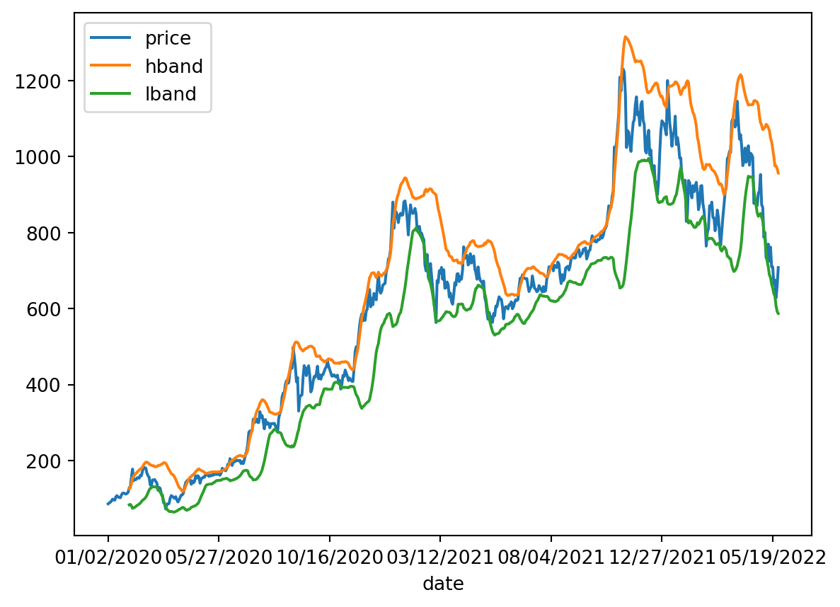

The following code is to create the following signal:

When the price is higher or equal to the “high (h)” band, it is a sell or short sell signal (-1). When the price is lower than the “low (l)” band, it’s a buy signal (1). Otherwise, it’s a neutral signal or doing nothing (0).

This is the “Loop For” for performing the procedure (getting the signals) for all the observations in the stock.

signal=[] 
for j in range(0,band_df.shape[0]): 

  # ----------this is rhe conditional for each observacion--------------

  if band_df["price"].iloc[j,] >= band_df["hband"].iloc[j,]:
      signal.append(-1) 
  elif band_df["price"].iloc[j,] <= band_df["lband"].iloc[j,]:
      signal.append(1) 
  else:
      signal.append(0) 
# ------------------------------------
signal[:5]

[0, 0, 0, 0, 0]

Here we print the result:

 signal_df=pd.DataFrame(signal,columns=["signal"])
 signal_df.plot()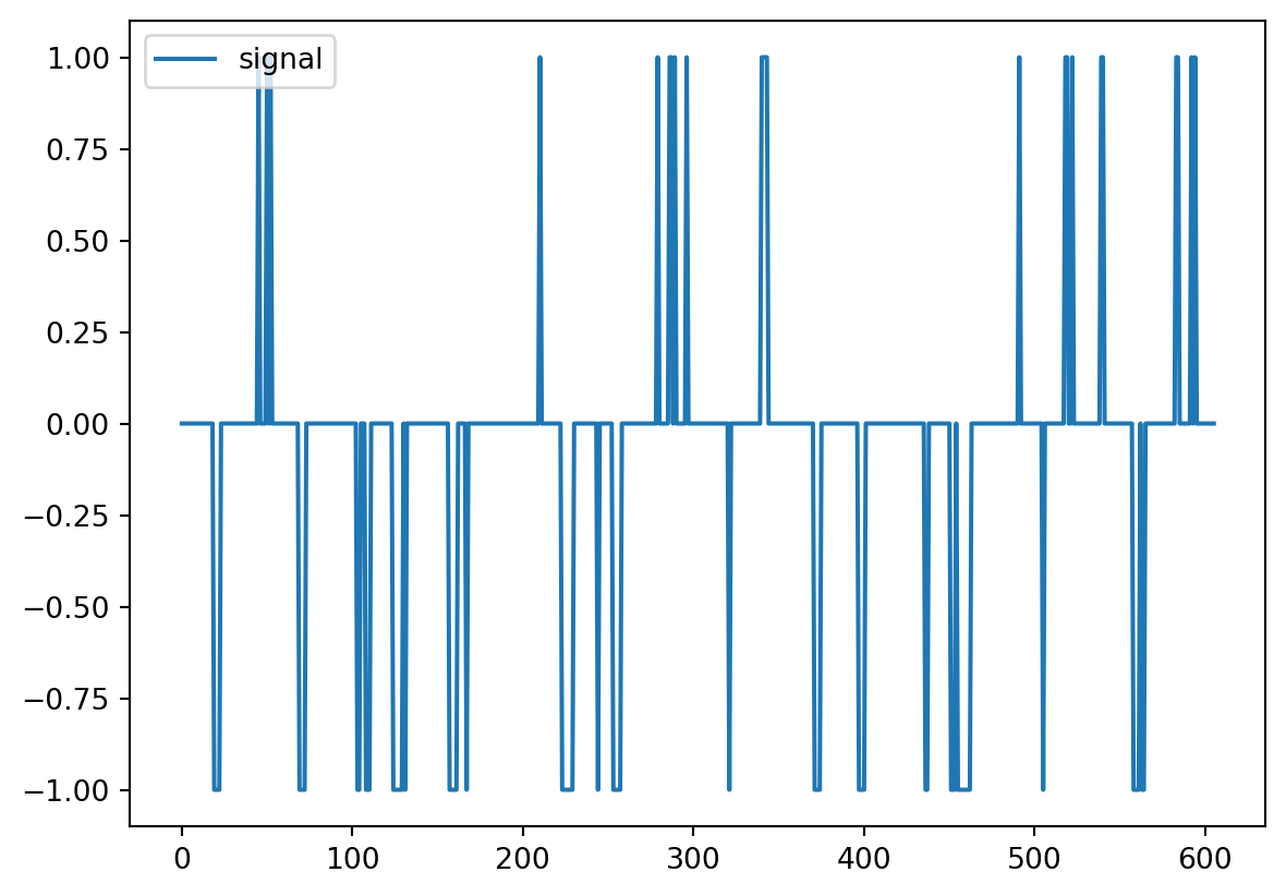

To estimate the strategy’s return, we will multiply the signal by the return for that day. We use the price of the signal day and the price one day after. Assuming it is a buying signal, we buy today and sell it tomorrow, making a one-day profit.

Then, the price of the signal day for observation 19 is:

j=19
band_df["price"].iloc[j,]

128.162003

The price of the day after is:

band_df["price"].iloc[j+1,]

130.113998

The associated signal for that observation:

signal_df["signal"].iloc[j,]

-1

The intuition for doing that is: If the signal is one(minus one), it means that the strategy was to buy (sell or short sale) the stock that day and sell (buy) it the next day. If the return is positive (negative), then it implies that the stock price increased (decreased), and by multiplying the return with the signal, we validate that the return of our strategy is positive.

On the contrary, if the signal is one (minus one) and the return negative (positive), it would imply that the price decreased (increased), and by buying (selling or short selling) the stock, we would have a loss, which is represented by the negative return.

Finally, if the signal is zero and the return is positive (negative), the result will be zero, implying that we did not buy (sell) the stock and didn’t have a return for that.

((band_df["price"].iloc[j+1,]/band_df["price"].iloc[j,])-1)*signal_df["signal"].iloc[j,] # el rendimiento aritmético

-0.015230684245782333

The previous is a daily return. Also, that procedure is for one signal, but we are looking for the return of all signals.

The next code is to get the location of all signals inside signal_df

sig_ret=[]
for i in range(signal_df.shape[0]):
    if signal_df["signal"].iloc[i,] != 0: # for signals different than 1 or -1
      sig_ret.append(i) 
sig_ret[:5]

[19, 20, 21, 22, 45]

The following code estimates the daily return strategy for each signal multiplied by the signal.

ret_i=[]
for j in sig_ret:
  ret_i.append(((band_df["price"].iloc[j+1,]/band_df["price"].iloc[j,])-1)*signal_df["signal"].iloc[j,])
 
ret_i[:5]

[-0.015230684245782333,
 -0.19894863272128482,
 -0.13725642948717942,
 0.1717583956255767,
 0.061397994430888]

The previous are daily returns. Here, we estimate the strategy annualized return for this stock as the average return.

ret=pd.DataFrame(ret_i,columns=["ret"]) 

pow((1+ret.mean().loc["ret",]),252)-1

-0.9083067491493413

The next step is to create a “Loop For” to perform the same procedure we did for Tesla for all stock inside data and store the results in a data frame.

ret_all=[] 
for ticker in data.columns:
  bb=ta.volatility.BollingerBands(data[ticker], window=20, window_dev=2)
  hb=bb.bollinger_hband() 
  lb=bb.bollinger_lband() 
  band_df=data[ticker]
  band_df=pd.concat([band_df,hb,lb],axis=1)
  band_df.columns=["price","hband","lband"]
  signal=[]
  for j in range(0,band_df.shape[0]-1): ## There are 983 rows in this case, and we have to 
        #limit ourselves to observation 982. If there is a signal in row 983, we cannot estimate 
        #the return because we need the price of the day after, and there is no day after. 
    if band_df["price"].iloc[j,] >= band_df["hband"].iloc[j,]:
      signal.append(-1) 
    elif band_df["price"].iloc[j,] <= band_df["lband"].iloc[j,]:
        signal.append(1) 
    else:
        signal.append(0) 
  signal_df=pd.DataFrame(signal,columns=["signal"])
  sig_ret=[]
  for i in range(signal_df.shape[0]):
      if signal_df["signal"].iloc[i,] != 0: 
          sig_ret.append(i) 
  ret_i=[]
  for j in sig_ret:
    ret_i.append(((band_df["price"].iloc[j+1,]/band_df["price"].iloc[j,])-1)*signal_df["signal"].iloc[j,])
  ret=pd.DataFrame(ret_i,columns=["ret"]) 
  ret_all.append(pow((1+ret.mean().loc["ret",]),252)-1) # 
ret_df=pd.DataFrame(ret_all,index=data.columns,columns=["ret"]).sort_values(by="ret",ascending=True) 
ret_df.head()

	ret
TSLA.Close	-0.908307
WFC.PL.Close	-0.601139
BML.PH.Close	-0.585364
BML.PL.Close	-0.447650
BAC.PE.Close	-0.367621

ret_df.tail()

	ret
TCTZF.Close	16.205044
BABAF.Close	20.254857
LRLCF.Close	45.638141
CICHF.Close	55.355042
RHHBF.Close	408.653265

As we can see, returns range from -0.908307 to 408.65. The following filter is to keep the stocks for which the strategy return is higher than 10% (0.1).

ret_filt=ret_df[ret_df["ret"]>.10]
ret_filt.head()

	ret
COST.Close	0.133845
CSCO.Close	0.162942
WFC.PY.Close	0.186977
XOM.Close	0.206523
CVX.Close	0.212237

Finally, we store the prices of those stocks only with a strategy return higher than a threshold, in this case, 10%.

data2=data.loc[:,ret_filt.index]
data2.head()

	COST.Close	CSCO.Close	WFC.PY.Close	XOM.Close	CVX.Close	JPM.PD.Close	PG.Close	SHEL.Close	RYDAF.Close	NKE.Close	...	TMUS.Close	NVSEF.Close	INTC.Close	PEP.Close	TCEHY.Close	TCTZF.Close	BABAF.Close	LRLCF.Close	CICHF.Close	RHHBF.Close
date
01/02/2020	291.489990	48.419998	26.870001	70.900002	121.430000	27.639999	123.410004	59.740002	30.000000	102.199997	...	78.589996	94.800003	60.840000	135.820007	49.880001	49.880001	27.25	293.450012	0.87	324.950012
01/03/2020	291.730011	47.630001	26.850000	70.330002	121.010002	27.660000	122.580002	60.209999	30.180000	101.919998	...	78.169998	93.250000	60.099998	135.630005	49.029999	48.930000	26.91	297.130005	0.84	319.750000
01/06/2020	291.809998	47.799999	26.840000	70.870003	120.599998	27.580000	122.750000	60.959999	30.469999	101.830002	...	78.620003	94.349998	59.930000	136.149994	48.770000	48.700001	26.91	293.000000	0.84	319.750000
01/07/2020	291.350006	47.490002	26.570000	70.290001	119.059998	27.500000	121.989998	60.400002	30.549999	101.779999	...	78.919998	95.000000	58.930000	134.009995	49.779999	49.770000	26.91	288.549988	0.88	322.049988
01/08/2020	294.690002	47.520000	26.580000	69.230003	117.699997	27.549999	122.510002	59.689999	30.139999	101.550003	...	79.419998	94.720001	58.970001	134.699997	49.650002	49.650002	26.91	287.500000	0.88	322.049988

5 rows × 46 columns